Cut Set Analysis
FaultTree User's Tutorial
TOC
*** This page has proven to be the most read of all in this tutorial. Indeed this is an important component of fault tree analysis. It has been years since this tutorial was originally written and currently with FaultTree released on CRAN there has been much enhancement of the cutsets function. Users may note that the default behavior of the cutsets function is to render the cutsets according to tag strings, rather than ID number. This behavior can be reset to correspond with the text by adding an argument by="id". Also the enhanced, more stable, code has been implemented in C++ for performance. This was never intended to obscure the method to users familiar with R, so a separate package is available on github that provides the function as implemented in easier to read, and single step perhaps. https://github.com/jto888/FaultTree.reference Readers will also find in that package prototype code in R for the BDD implementation for prime implicants. Keep in mind comments are always welcome.
****
Cut Set Analysis
During the development of fault trees there are times when a basic event entry for the same component with the same failure mode appears in more than one position in the tree. This occurs so frequently that the term Multiply Occurring Event (MOE) is widely used. At times replication may involve an entire branch of a tree as a Multiply Occurring Branch (MOB), in which case all component events comprising the duplicated branch are MOE's.
Depending on the design of the fault tree structure, or when a team of participants works on the same large tree, MOE's may be distributed under one or more AND gates. Such occurrences may hide the true significance of certain events, rendering inaccuracies when the tree is calculated on a bottom-up, gate-by-gate fashion as the FaultTree::ftree.calc function does.
Cut set analysis is widely performed to mitigate these risks in fault tree construction. A cut set is a distinct path of failure leading to the top undesired event. Upon initial dissection of a fault tree many cut sets are typically identified, but not all are unique. Repeated combinations of events may also be found in cut sets having the same number of events combined by an AND operation. A process of reduction using the laws of Boolean algebra is then applied to identify only the truly unique minimal cut sets.
Several algorithms have been identified for methodically identifying all cut sets in a fault tree and then reducing them to the minimal cut sets. The FaultTree package has currently implemented only one of the popular early algorithms referred to as Method for Obtaining CUt Sets (MOCUS). This is perhaps implemented as a demonstration, rather than production level code and is known to be in need of additional debugging. As a pure R implementation for this algorithm the source code is perhaps the best documentation for those interested in exploring this further. Since this is an open source effort all are encouraged to make this a study. For purposes of this discussion an example will be worked out to demonstrate the use.
The chosen example has been obtained from Appendix B of Clifton Ericson's "Fault Tree Analysis Primer" available for purchase at: https://www.amazon.com/Fault-Analysis-Primer-Clifton-Ericson/dp/1466446102

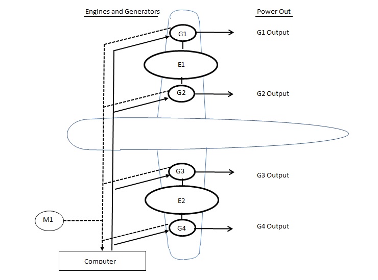
Presume a hypothetical power generation system driven off of a dual engine aircraft. Each engine can drive either or both generators associated with it, although one on each wing is initially a stand-by. Two of the total four generators must operate to produce sufficient power. A computer on the aircraft is responsible for identifying failure of any running generator and switching to a stand-by so as to avoid power failure. The undesired event is insufficient power. This will occur if 3 out of 4 generators cannot produce power.
As sometimes happens during group study a consensus (or simply the loudest or highest ranking voice in the room) may focus first on the 3 out of 4 generator combinations that would result in insufficient power. Then, the fault tree is completed by analyzing the causal flow of events for for failure of each generator output back-to-front. Resulting in a fault tree generated by the following script.
pwr<-ftree.make(type="or", name="insufficient", name2="Electrical Power")
pwr<-addLogic(pwr, at=1, type="and", name="No Output", name2="G1, G2, G3")
pwr<-addLogic(pwr, at=2, type="or", name="No Power", name2="From G1")
pwr<-addLogic(pwr, at=3, type="or", name="No Output", name2="From G1")
pwr<-addProbability(pwr, at=3, prob=1e-4, tag="G1A", name="G1 Conn Open")
pwr<-addProbability(pwr, at=4, prob=1e-3, tag="G1", name="Generator G1", name2="Fails")
pwr<-addLogic(pwr, at=4, type="or", name="No Input", name2="To G1")
pwr<-addProbability(pwr, at=7, prob=1e-3, tag="E1", name="Engine E1", name2="Fails")
pwr<-addProbability(pwr, at=7, prob=1e-4, tag="G1B", name="Bleed Air To", name2="G1 Fails")
pwr<-addLogic(pwr, at=2, type="or", name="No Power", name2="From G2")
pwr<-addProbability(pwr, at=10, prob=1e-4, tag="G2A", name="G2 Conn Open")
pwr<-addLogic(pwr, at=10, type="or", name="No Output", name2="From G2")
pwr<-addLogic(pwr, at=12, type="or", name="No Input", name2="To G2")
pwr<-addDuplicate( pwr, at=13, dup_id=8)
pwr<-addProbability(pwr, at=13, prob=1e-4, tag="G2B", name="Bleed Air To", name2="G2 Fails")
pwr<-addProbability(pwr, at=12, prob=1e-3, tag="G2", name="Generator G2", name2="Fails")
pwr<-addLogic(pwr, at=12, type="or", name="Switch To", name2="G2 Fails")
pwr<-addProbability(pwr, at=17, prob=1e-4, tag="M1", name="Monitor M1", name2="Fails")
pwr<-addProbability(pwr, at=17, prob=1e-4, tag="S1", name="Switching S1", name2="Fails")
pwr<-addLogic(pwr, at=2, type="or", name="No Power", name2="From G3")
pwr<-addLogic(pwr, at=20, type="or", name="No Output", name2="From G3")
pwr<-addProbability(pwr, at=20, prob=1e-4, tag="G3A", name="G3 Conn Open")
pwr<-addProbability(pwr, at=21, prob=1e-3, tag="G3", name="Generator G3", name2="Fails")
pwr<-addLogic(pwr, at=21, type="or", name="No Input", name2="To G3")
pwr<-addProbability(pwr, at=24, prob=1e-3, tag="E2", name="Engine E2", name2="Fails")
pwr<-addProbability(pwr, at=24, prob=1e-4, tag="G3B", name="Bleed Air To", name2="G2 Fails")
pwr<-addLogic(pwr, at=1, type="and", name="No Output", name2="G1, G2, G4")
pwr<-addDuplicate( pwr, at=27, dup_id=3)
pwr<-addDuplicate( pwr, at=27, dup_id=10)
pwr<-addLogic(pwr, at=27, type="or", name="No Power", name2="From G4")
pwr<-addProbability(pwr, at=45, prob=1e-4, tag="G4A", name="G4 Conn Open")
pwr<-addLogic(pwr, at=45, type="or", name="No Output", name2="From G4")
pwr<-addLogic(pwr, at=47, type="or", name="No Input", name2="To G4")
pwr<-addDuplicate( pwr, at=48, dup_id=25)
pwr<-addProbability(pwr, at=48, prob=1e-3, tag="G4", name="Generator G4", name2="Fails")
pwr<-addProbability(pwr, at=47, prob=1e-4, tag="G4B", name="Bleed Air To", name2="G4 Fails")
pwr<-addLogic(pwr, at=47, type="or", name="Switch To", name2="G4 Fails")
pwr<-addDuplicate( pwr, at=52, dup_id=18)
pwr<-addDuplicate( pwr, at=52, dup_id=19)
pwr<-addLogic(pwr, at=1, type="and", name="No Output", name2="G1, G3, G4")
pwr<-addDuplicate( pwr, at=55, dup_id=3)
pwr<-addDuplicate( pwr, at=55, dup_id=20)
pwr<-addDuplicate( pwr, at=55, dup_id=45)
pwr<-addLogic(pwr, at=1, type="and", name="No Output", name2="G2, G3, G4")
pwr<-addDuplicate( pwr, at=80, dup_id=10)
pwr<-addDuplicate( pwr, at=80, dup_id=20)
pwr<-addDuplicate( pwr, at=80, dup_id=45)
And viewed with:
ftree2html(pwr, write_file=TRUE)
browseURL("pwr.html")
With a zoom out to 50% and some strategic node collapses of duplicated branches it is possible to contain the content of this tree in a single view. The FaultTree package does not currently support transfer gates; however the ability to produce different views by expand or collapse on nodes appears to provide a sufficient work-around.
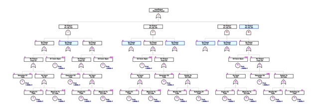
The script for this tree makes considerable use of the addDuplicate function, which does what is its name suggests. Both source and duplicated nodes are modified with magenta coloring for several attributes. For a source node an 'S' is placed at the upper left of the label box. An 'R' appears in this position for a repeated node. For repeated nodes the ID of the source is shown in the gate graphic rather than its actual node ID. This should not present a problem for identifying the placement of further nodes, since connections to sources or repeated nodes is not permitted once a duplication has been made.
Probability values have been provided in this example, while none were listed in the book example. An order of magnitude was chosen to distinguish complex assemblies (engine or generator) from individual components (switches, valves, relays, etc.). It is trusted that all of these values are pessimistic, else no one would want to fly in aircraft. Calculation is not performed yet, as we wish to examine the cut set analysis first.
The ftree.cutsets function will return the minimal cut sets for the named fault tree in a list of matrix objects. In addition to viewing this output it will be desirable to perform more manipulations. For this reason the output is assigned to an object name, 'pwr_cs' in this case. The command line is:
&tbsp;
pwr_cs<-cutsets(pwr)
Users may note that since the original CRAN release of FaultTree version .995 the default behavior of the cutsets function is to render the cutsets according to tag strings, rather than ID number. This behavior can be reset to correspond with the text below by adding an argument by="id".
pwr_cs<-cutsets(pwr,by="id")
Now, viewing the pwr_cs object reveals an output described as follows:
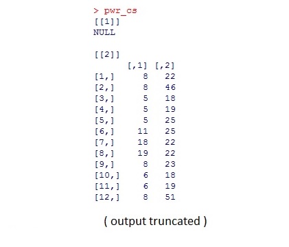
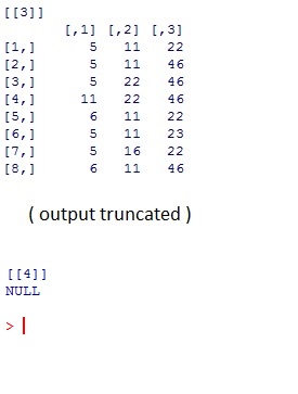
This output is a list of matrices. The numerical order of the list items in double braces "[ [ # ] ]" indicates the order, or number of elements in the listed cut sets. Here there are no single order cut sets and no 4th order cut sets. The values shown in the matrices are node ID's. Each row represents nodes combined by AND logic. For any duplicated nodes the ID is taken from the source of duplication. Here the actual output is truncated; however by scrolling through the output in the R Console it is quickly determined that there are 29 second order cut sets and 108 third order cut sets. This is good because it is exactly what Clifton Ericson also found.
At this point the packaged code has identified the minimal cut sets, but the output is not yet in most useful form. The next few steps will utilize the R environment to manipulate the output as desired. Since we know that tags have been provided for all basic events in this example, it would be nice to translate the cut set matrices to show tags. This kind of operation across an entire matrix is facilitated by an apply function in R. After each operation it is recommended to view the object created by typing just the object name and enter. This will confirm what is going on. For those particularly interested, get the help pages ?apply and ?which to gain understanding on how this works.
To get the tags for each element of the cut sets enter the following code:
cs_tags2<-apply(pwr_cs[[2]], c(1,2),function(x) pwr$Tag[which(pwr$ID==x)])
cs_tags3<-apply(pwr_cs[[3]], c(1,2),function(x) pwr$Tag[which(pwr$ID==x)])
Similarly, it would be handy to have the probability values for each of the elements of the cut sets.
cs_probs2<-apply(pwr_cs[[2]], c(1,2),function(x) pwr$PBF[which(pwr$ID==x)])
cs_probs3<-apply(pwr_cs[[3]], c(1,2),function(x) pwr$PBF[which(pwr$ID==x)])
Since each row of the cut set represents a single probability resulting from the product of its elements, it is possible to build a probability column to add to the cut set tags now as a dataframe.
cs_tags2<-cbind(cs_tags2, data.frame('prob'=apply(cs_probs2, 1, function(x) prod(x))))
cs_tags3<-cbind(cs_tags3, data.frame('prob'=apply(cs_probs3, 1, function(x) prod(x))))
[R details - There is a bit of sleight-of-hand going on at this point. Since the cs_tags matrices contained all character entries, and we wish to add a numeric column we have to force the new cs_tags objects to be dataframes. Dataframes can hold different object types as long as the columns have consistent types within.]
Now, it would be nice to combine these dataframes and order the cut sets according to probability (decreasing) and tag text values (increasing). First, a column of empty values (NA) must be added to cs_tags2 to give same number of rows as cs_tags3. Then the column names need to assigned as the same . Finally the two objects can be combined to one and sorted (ordered). Lastly, the rows are re-numbered for ascetics.
nas<-rep(NA,length(cs_tags2[,1]))
cs_tags2<-cbind(cs_tags2[,1:2],nas, cs_tags2[,3])
names(cs_tags2)<-names(cs_tags3)
all_cs<-rbind(cs_tags2, cs_tags3)
all_cs<-all_cs[order(-all_cs[,4],all_cs[,1], all_cs[,2], all_cs[,3],na.last=FALSE), ]
row.names(all_cs)<-as.character(1:length(all_cs[,1]))
The resulting 'all_cs' dataframe provides a simplistic importance view of all of the cut sets, since it ranks according to the probability of each distinct path to failure.
To be honest the ftree.cutsets function should incorporate the above steps so as to return such an importance view object directly. This will require coding the steps detailed in this section into the FaultTree source. However there are still unanswered questions as to how so called, non-coherent, trees built on the repairable system model should be handled. Currently all specialty gates will be treated as AND combinations and effort is required to restore full description of each cut set. For now this is left for analyst interpretation using the R environment.
Now, this example can be calculated by taking the probabilistic sum of all unique, minimal cut set probabilities. This is considered the Minimal Cutsets Upper Bound (MCUB) approximation. It is an approximation because further consideration of the effect of multiple occurrences of duplicated basic events has not been made.
> 1-prod(1-all_cs$prob)
[1] 6.686892e-06
The original fault tree could be calculated as in the past. The specific dataframe entry for the probability of the top event then requested for return:
> pwr <-ftree.calc(pwr)
> pwr$PBF[1]
[1] 4.847278e-08
What happened? Calculation of the example tree according to gate-by-gate calculations reveals a significant deviation!
The original fault tree was constructed under the assumption that the generation of power was based purely on a 2 out of 4 redundancy of generators. Once initiated down this path the generation of second order events leading to the top event became unlikely. Clearly, from a causal perspective if both engines fail there would be no means for generation of power. Likewise, if a single engine were to fail and one of the generators on the other side were to fail only one generator would remain available. Finally, if either engine or any operating generator were to fail there would be a dependency on the computer and switching systems to activate a stand-by. These cases were specifically modeled in a causal fashion during construction of the original fault tree. It is almost magical that the cut set analysis is able to identify these events.
The situation demonstrated by this example has lead some practitioners to eschew gate-by-gate calculation whatsoever. In reality it appears that fault tree practitioners should be aware of the risks and utilize cut set analysis to check their work. One could argue that much of this risk is due to inaccurate fault tree construction; however, cut set analysis is available to aid in checking such oversights and is invaluable for that purpose.
It is left as a student exercise to build an alternative fault tree based on the knowledge gained through cut set analysis. Start with a causal approach rather than functional. A faithfully developed solution will result in the same minimal cutsets, but likely produce close agreement with the MCUB upon gate-by-gate calculation.
TOC
NEXT -->