Advanced Calculations for PRA

Fault tree construction, quantification of basic-event elements and ultimately calculation of top event probability is foundational to Probabilistic Risk Analysis (PRA). In the previous example it has been observed that only approximations of the top event probability could be made, given a tree containing considerable entries of Multiply Occurring Events (MOE). The base functions in the FaultTree package for R have not been developed to handle the full range of required calculations for PRA. Fortunately, a compliment to this package is available through same GPL open source licensing to make these calculations available.

SCRAM is a Command-line Risk Analysis Multi-tool. A complimentary package to FaultTree, named FaultTree.SCRAM provides functions to call scram on the ftree object created by FaultTree to obtain advanced calculations for PRA. These new software items need separate installation.

Installation instructions for various operating systems are available from the scram-pra.org site. For Windows users a pre-compiled binary installer is available on SourceForge. Once installed, the PATH environment variable needs to include an entry for the /bin folder where scram.exe exists.

The FaultTree.SCRAM package is available on the same R-Forge repository where the FaultTree package exists. Its installation follows the same steps as covered in the Introduction to this tutorial.

A single call to load the FaultTree.SCRAM package into a new R instance will also load the dependent FaultTree package.

library(FaultTree.SCRAM)

Now load the pwr script from the previous Cut Set Analysis page. Then a simple call can be made to get the exact probability for the top event.

scram.probability(pwr)

This is the accepted “exact” probability obtained by Binary Decision Diagram (BDD). Additional reading on this is encouraged on the scram-pra.org site.

Additional commands that can be made on this model are:

scram.cutsets(pwr)

scram.probability(pwr, list_out=TRUE)

scram.importance(pwr)

The final command introduced here produces an output of 5 different importance measures on the basic-events as found in the literature. These are enumerated in the help page for this command and repeated here:

Fussel-Vesely Diagnosis Importance Factor (DIF)
Birnbaum Marginal Importance Factor (MIF)
Critical Importance Factor (CIF)
Risk Reduction Worth (RRW)
Risk Achievement Worth (RAW)

Fault Tree Example pwr Revisited

Revisiting the student exercise from the Cut Set Analysis page, the following script for the first part of a revised pwr fault tree is provided:

pwr2a<-ftree.make(type="or", name="insufficient", name2="Electrical Power")
pwr2a<-addLogic(pwr2a, at=1, type="and", name="Both Engines", name2="Fail")
pwr2a<-addProbability(pwr2a, at=2, prob=1e-3, tag="E1", name="Engine E1", name2="Fails")
pwr2a<-addProbability(pwr2a, at=2, prob=1e-3, tag="E2", name="Engine E2", name2="Fails")
pwr2a<-addLogic(pwr2a, at=1, type="and", name="Events Dependent on", name2="Monitoring and Switching")
pwr2a<-addLogic(pwr2a, at=5, type="or", name="Single Primary", name2="Unit Failure")
pwr2a<-addLogic(pwr2a, at=6, type="or", name="Single Engine", name2="Failure")
pwr2a<-addDuplicate(pwr2a, at=7, dup_id=3)
pwr2a<-addDuplicate(pwr2a, at=7, dup_id=4)
pwr2a<-addLogic(pwr2a, at=6, type="or", name="Single Primary", name2="Gen Failure")
pwr2a<-addLogic(pwr2a, at=10, type="or", name="Primary Generation", name2="Failure Side 1")
pwr2a<-addProbability(pwr2a, at=11, prob=1e-3, tag="G2", name="Generator G2", name2="Fails")
pwr2a<-addProbability(pwr2a, at=11, prob=1e-4, display_under=12, tag="G2A", name="G2 Conn Open")
pwr2a<-addProbability(pwr2a, at=11, prob=1e-4, display_under=13, tag="G2B", name="Bleed Air To", name2="G2 Fails")
pwr2a<-addLogic(pwr2a, at=10, type="or", name="Primary Generation", name2="Failure Side 2")
pwr2a<-addProbability(pwr2a, at=15, prob=1e-3, tag="G4", name="Generator G4", name2="Fails")
pwr2a<-addProbability(pwr2a, at=15, prob=1e-4, display_under=16, tag="G4A", name="G4 Conn Open")
pwr2a<-addProbability(pwr2a, at=15, prob=1e-4, display_under=17, tag="G4B", name="Bleed Air To", name2="G4 Fails")
pwr2a<-addLogic(pwr2a, at=5, type="or", name="Monotor or Switching", name2="Fails")
pwr2a<-addProbability(pwr2a, at=19, prob=1e-4, tag="M1", name="Monitor M1", name2="Fails")
pwr2a<-addProbability(pwr2a, at=19, display_under=20, prob=1e-4, tag="S1", name="Switching S1", name2="Fails")
pwr2a<-addLogic(pwr2a, at=1, type="or", name="Single Engine Fail with", name2="Generation Loss Other Side")
pwr2a<-addLogic(pwr2a, at=22, type="and", name="Engine E1 Fail with", name2="Generation Loss Side 2")
pwr2a<-addDuplicate(pwr2a, at=23, dup_id=3)
pwr2a<-addLogic(pwr2a, at=23, type="or", name="Generation Loss", name2="Side 2")
pwr2a<-addDuplicate(pwr2a, at=25, dup_id=15)
pwr2a<-addLogic(pwr2a, at=25, type="or", name="StandBy Generation", name2="Failure Side 2")
pwr2a<-addProbability(pwr2a, at=30, prob=1e-3, tag="G3", name="Generator G3", name2="Fails")
pwr2a<-addProbability(pwr2a, at=30, prob=1e-4, display_under=31, tag="G3A", name="G3 Conn Open")
pwr2a<-addProbability(pwr2a, at=30, prob=1e-4, display_under=32, tag="G3B", name="Bleed Air To", name2="G3 Fails")
pwr2a<-addLogic(pwr2a, at=22, type="and", name="Engine E2 Fail with", name2="Generation Loss Side 1")
pwr2a<-addDuplicate(pwr2a, at=34, dup_id=4)
pwr2a<-addLogic(pwr2a, at=34, type="or", name="Generation Loss", name2="Side 2")
pwr2a<-addDuplicate(pwr2a, at=36, dup_id=11)
pwr2a<-addLogic(pwr2a, at=36, type="or", name="StandBy Generation", name2="Failure Side 1")
pwr2a<-addProbability(pwr2a, at=41, prob=1e-3, tag="G1", name="Generator G1", name2="Fails")
pwr2a<-addProbability(pwr2a, at=41, prob=1e-4, display_under=42, tag="G1A", name="G1 Conn Open")
pwr2a<-addProbability(pwr2a, at=41, prob=1e-4, display_under=43, tag="G1B", name="Bleed Air To", name2="G1 Fails")

A quick check confirms that this tree generates the same 29 second-order minimal cut sets as the original pwr model.

scram.cutsets(pwr2a)

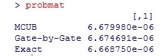
Now estimates for probability of these most significant contributors to the pwr top event can be produced:

pwr2a_mcub<-1-(prod(1-scram.probability(pwr2a, list_out=T)[[2]][3]))
pwr2a_gbg<-ftree.calc(pwr2a)$PBF[1]
pwr2a_exact<-scram.probability(pwr2a)
pwr2a_prob<-c(pwr2a_mcub,pwr2a_gbg,pwr2a_exact)
probmat<-as.matrix(pwr2a_prob)
rownames(probmat)<-c("MCUB","Gate-by-Gate","Exact")
probmat

Now it is observed that the gate-by-gate calculation is producing a result in close agreement with the MCUB and the exact value. With a certain arrangement of the fault tree this method is certainly valid. Indeed this grouping of basic elements under OR gates prior to AND mimics the Esary-Proschian approximation. Additionally the probability values that can now be observed for the causal gates feeding the top event reveal vulnerabilities of the system in a quantified way.

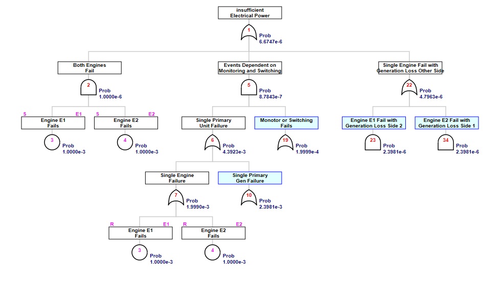
While it is frightening to think of dual engine failure, it might be surprising to note that over half of the risk of power failure in this example starts with a single engine failure. No wonder Sully had an "APU" to turn on during the "Miracle on Hudson" event. Most engineers will also note that redundancy in the singular system for monitoring and switching would be most cost effective in reducing risk.

Since it was previously found that the MCUB for the full pwr top event was 6.686892e-06, it can reasonably be expected that the impact of the 3 out of 4 generation systems in failure will be on the order of 6.9e-09. Quite a modest contribution indeed for these 108 third-order cutsets.

The SCRAM program provides an implementation of an 'atleast' gate for simplifying tree construction for such voting type combinations. The complete alternate tree can now be constructed as:

## assign the previous partial tree to a new object label
pwr2<-pwr2a
pwr2<-addAtLeast(pwr2, at=1, atleast=3, name="At Least 3 Gen", name2="Sytems Fail")
pwr2<-addDuplicate(pwr2, at=45, dup_id=41)
pwr2<-addDuplicate(pwr2, at=45, dup_id=11)
pwr2<-addDuplicate(pwr2, at=45, dup_id=30)
pwr2<-addDuplicate(pwr2, at=45, dup_id=15)

Here is a view displaying detail for just the 'atleast' gate:

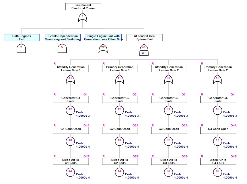
Note that the ftree.calc function cannot resolve this 'atleast' gate. In the RAM modeling system, to be discussed later, a VOTE gate could be used to accomplish similar simplification. However, SCRAM will not resolve that formulation.

Handling Uncertainty

The analysis risk in statistical fashion is indeed a study of uncertainty. Unfortunately the data for basic event elements is often a crude approximation, or at best the mean of some distributed data.To provide insight into the effect of uncertain input data, SCRAM has implemented the random deviates defined in the MEF Stochastic Layer. To date the FaultTree.SCRAM package has implemented three of these MEF random deviates; uniform, normal and the somewhat unconventional lognormal defined by mean, error factor, and confidence level parameters. Additional random deviates will be implemented as they are tested further.

Uncertainty is applied to mean parameters of the basic element, currently only the mean probabiility, or the lambda value of an exponentially exposed event. This application of uncertainty has no effect on other functionalities (calculations, cutset determinations, importance, or display) of the fault tree object, but is required to define the input for analysis by scram.uncertainty. The application of uncertainty is demonstrated by applying a normal deviate to the probability values of the complex assemblies (engine or generator) in the pwr2 example using applyUncertainty function that can be appended to the end of a FaultTree script.

pwr2<-applyUncertainty(pwr2, on=3, what="prob", deviate="normal", param=1.6e-4)
pwr2<-applyUncertainty(pwr2, on=4, what="prob", deviate="normal", param=1.6e-4)
pwr2<-applyUncertainty(pwr2, on=12, what="prob", deviate="normal", param=1.6e-4)
pwr2<-applyUncertainty(pwr2, on=16, what="prob", deviate="normal", param=1.6e-4)
pwr2<-applyUncertainty(pwr2, on=31, what="prob", deviate="normal", param=1.6e-4)
pwr2<-applyUncertainty(pwr2, on=42, what="prob", deviate="normal", param=1.6e-4)

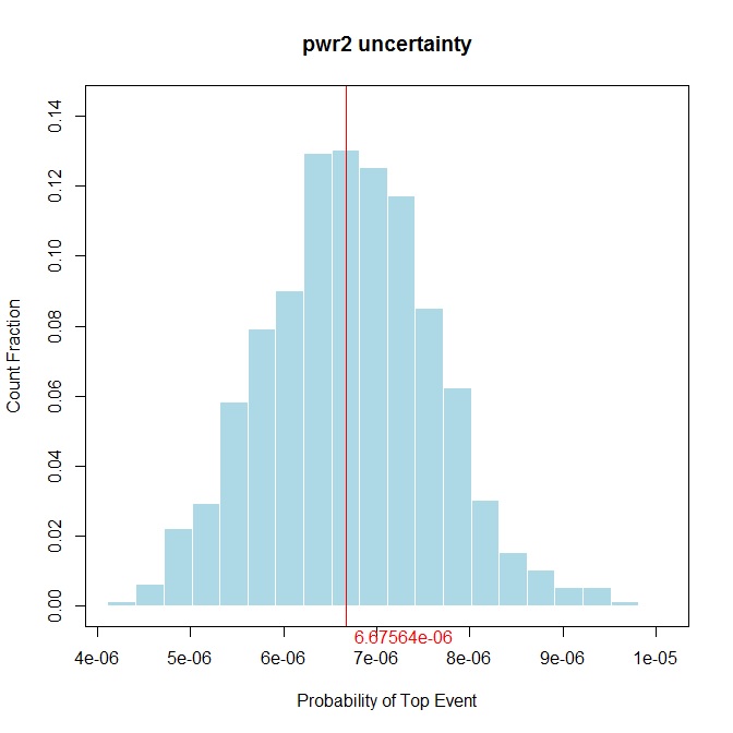
Now a call can be made to acquire the SCRAM uncertainty analysis with a graphical display of the histogram of "Exact" probabilities (by BDD) of the top event through the stochastic trials.

pwr2_unc<-scram.uncertainty(pwr2, show=c(T,F))

TOC
NEXT -->