Using abrem

Functions of the abrem package provide an application layer for entering life data, selecting various options for the treatment of that data, generation of a graphical display, and presenting meaningful statistical output in a legend. This application layer is executed in the R console, based on scripts that are likely prepared in a separate editor.

Package abrem makes use of the R object model to prepare objects for plotted output. Various options are handled to extend the object with parametric fitting, preparation of confidence interval bounds, and preparation of the graphical output.

Preliminary steps for using abrem involve installing the package and its dependencies into your R system. This topic is discussed separately in the How-To page. 

For a rapid Weibull 2-parameter fit and display, an object is constructed using the Abrem() function on the data of interest. Then a fit element is added using object method abrem.fit(). This object can then be plotted with the R function plot(). To demonstrate this simple use, the initial problem sets from Chapter 2 of “The New Weibull Handbook” are shown below. 

For each example copy the code script in the gray shaded area and paste it into the R Console to execute and view as intended.

library(abrem)
Prob2.1Data<-c(150,85,250,240,135,200,190) 
Prob2.1Object<-Abrem(Prob2.1Data)
Prob2.1Object<-abrem.fit(Prob2.1Object)
plot(Prob2.1Object, main="Problem 2-1")

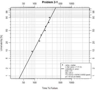
This is a first, simple, plotting example. In the script above the first line merely assures that the abrem package and all its dependencies have been loaded in this R session. 

The second line places the example data into a vector. 

The third line uses function Abrem() to construct an abrem object from the data. The Abrem function has been designed for some flexibility of data input. In this case, a single numeric vector has been passed as the first argument, so it is taken to be a set of complete failure times. This initial object could have been plotted at this point and one would observe the points, only, plotted on the default canvas for a Weibull analysis. Since we are using the default options.abrem list, the plotting distribution is “weibull2p”, and the plotting positions have been determined using the beta binomial function for most technically accurate median rank positions. These positions are minimally different than the Benard approximation method used in the “Handbook” text.

The fourth line of the script adds a fit of the data into the abrem object using the abrem.fit() method on the object. According to defaults of the options.abrem list, this fit is by rank regression using the preferred X on Y ordering convention.

Finally, the fifth line plots the object based on the exposed elements of the abrem object, which has been provided as a first argument to the plot() function. In this case the main title of the chart has been specified. Upon execution of this line an R Graphics Device window is opened with the resulting display.

Now consider example Problem 2-2 from the text:

library(abrem)
Serials<-c(831,832,833,834,835,836,837,838)

Times<-c(9,6,14.6,1.1,20,7,65,8)
Events<-c(1,1,0,1,1,0,1,0)
Prob2.2Data<-data.frame(serial=Serials,
time=Times,event=Events)
Prob2.2Object<-Abrem(Prob2.2Data, col="red")
Prob2.2Object<-abrem.fit(Prob2.2Object)
plot(Prob2.2Object, main="Problem 2-2")

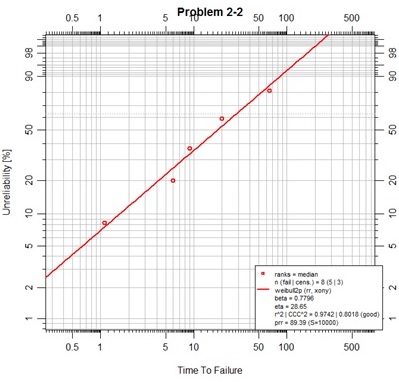
In the script above the data is entered into three vectors in the exact order as presented in a table in the text. These vectors are used to create a dataframe to present the data with specifically named fields of ‘time’ and ‘event’. Note that the event vector is made up of 1's for failures and 0's for suspensions. The Abrem() function will accept this format as a first argument. It will parse the dataframe for the two specifically named fields as shown singular and all lower case. Additional information that may be stored in the dataframe is not used on the abrem object that will be created by function Abrem(). In this example some color has been added to the object. A default rank regression fit is then added to the object as in the previous example. Finally the plot is executed providing a new main title for the chart.

library(abrem)
Prob2.1Data<-c(150,85,250,240,135,200,190)
Prob2.1Object<-Abrem(Prob2.1Data,
col="blue",label="Problem 2-1")
Prob2.1Object<-abrem.fit(Prob2.1Object)
P2.2Failures<-c(9.0,6.0,1.1,20.0,65.0)
P2.2Suspensions<-c(14.6,7.0,8.0)
Prob2.2Object<-Abrem(fail=P2.2Failures, susp=P2.2Suspensions,
col="red", label="Problem 2-2")
Prob2.2Object<-abrem.fit(Prob2.2Object)
title<-"Chapter 2 Problems"
plot.abrem(list(Prob2.2Object, Prob2.1Object), main=title)

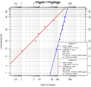
In this script some color is added to each problem object and identifying labels are added for the legend. The data for the second problem has been prepared for an alternate input means for object initialization by the Abrem() function. By this convention two vectors of time values are prepared; one for complete failures, the other for suspension data (also known as right-censored data). These two vectors must then be assigned to the specifically named arguments ‘fail’ and ‘susp’ in the Abrem() function call.

The procedure for placing two or more abrem objects into a chart is to pass the objects in a list to the plot.abrem() method. This is a special case for plotting abrem objects. The generic R plot() function cannot recognize such a list of abrem objects.

Continuing a convention of recalculating examples from our reference text, two examples are provided below plotting recalculations for Figure C-1 and Figure 7-5 (from Section 7.5.1) from the “New Weibull Handbook, Fifth Edition” below:

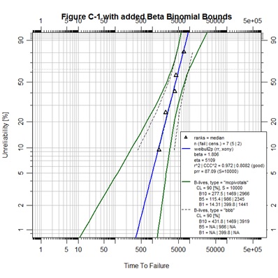
## Figure C-1
library(abrem)
AppBCData<-data.frame(
time=c(1500,1750,2250,4000,4300,5000,7000),
event=c(1,0,1,1,1,0,1))
FigC.1<-Abrem(AppBCData, pch=2)
FigC.1<-abrem.fit(FigC.1, col="blue")
FigC.1<-abrem.conf(FigC.1, col="darkgreen")
FigC.1<-abrem.conf(FigC.1, method.conf.blives="bbb",
lty=2, lwd=1, col="black")
plot(FigC.1, xlim=c(1,500000), ylim=c(.01,.90),
main="Figure C-1 with added Beta Binomial Bounds") 

The Figure C-1 script demonstrates graphic control over the individual elements of a single abrem object. During the object construction using Abrem() the point character, pch, is set to a value of 2 to generate upright triangles. By typing ?points in the R console a help page will appear in which all of the pch options are defined. As the default fit element is created it is assigned the color blue. As the default MCpivotal confidence bounds are created they are assigned a dark green color. Then, as a second confidence interval element is added as the beta binomial bounds, the line type, lty, and line width, lwd, are customized according to options that can be explored by typing ?par in the R console. So, it is demonstrated that each abrem object can have multiple elements and each of those elements can be graphically controlled.

A final observation can be noted in that the ranges for X and Y axes for Figure C-1 were altered to provide a more pleasing presentation than default code would have given.

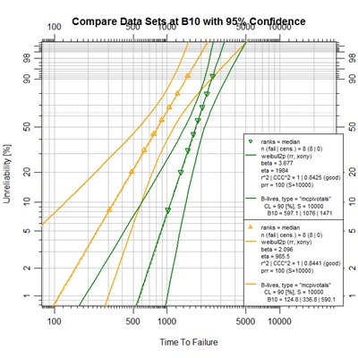
## Figure 7-5 (Section 7.5.1)
library(abrem)
set.seed(1234)
## function mrank is to be depreciated in favor of getPPP from abremPivotals
ppp<-getPPP(rep(1,8))[,2]
data1<-unlist(lapply(ppp,function℗qweibull(p,2.09,985.8)))
data2<-unlist(lapply(ppp,function℗qweibull(p,3.666,1984)))
Obj1<-abrem.conf(abrem.fit(Abrem(data1, pch=2, col="orange")), blives=0.1)
Obj2<-abrem.conf(abrem.fit(Abrem(data2, pch=6, col="forestgreen")), blives=0.1)
plot.abrem(list(Obj1,Obj2),
main="Compare Data Sets at B10 with 95% Confidence") 

The script for Figure 7-5 begins with a seed setting establishing a uniform state for the random number generator (RNG) as the function is called. This setting assures consistent numeric output of the Monte Carlo output regardless of any previous RNG activity. The next three lines establish ideal points for the given Weibull parameter pairs. This example demonstrates R’s lapply() function ability to loop through a vector of input values to a given function and return a list of output values. The qweibull() function returns the time value for a given Weibull parameter pair at a given unreliability percentage, this is called the quantile function. In this case, it was known that the result values were atomic vector elements, so the desired result was an unlist() of the output from lapply(). 

The two data sets, data1 and data2, are formed as vectors of complete failure time values. Then, a nested approach has been used to construct each object with all desired elements and their graphical features. Notice that the blives output was limited to a single report at B10 for this case. The blives option could have been set at any point in the construction of the objects in this case. Association with the abrem.conf just seemed most appropriate. Finally, as seen before, these objects were passed in a list to the object method plot.abrem() with a definition for the main chart title.

The point of this figure is to demonstrate a method of determining statistical distinctness of two data sets similar to a method presented in 1994 by Jim Lempke of Ford Motor Company. It is hard to see the distinction that exists at the B10 level (10% unreliability) between the upper bound of the orange set and the lower bound of the green set by the graph itself. It is hard to see this in the book also. However, the B-lives display in the legend clearly shows the 95% upper-bound B10 value to be 590.1 for the orange set, while the 95% lower-bound B10 value is 597.1 for the green set. Since the confidence limit, cl, has been defined as a 90% double-sided interval, the single-sided confidence levels are each 95%.

At this time preparation of pivotal confidence interval bounds for data sets with suspensions is a subject of some on-going study. The user is cautioned that bounds and B-Life determinations prepared for such abrem objects may be different than other software presentations. An open invitation is made here for participation in this study.

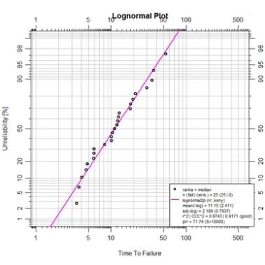
One of the few lognormal data examples from the text is provided in Figure
3-13.With the appropriate data entered into R as a vector named F3.13da the
following script can be run to generate the lognormal fit on the log-log canvas
for depicting linear regression.

library(abrem)
F3.13da <- c(3.46623, 3.732711,
4.052996, 4.628703, 4.8157,
5.84517, 5.888313, 5.892967,
8.168362, 10.02799, 10.06062,
10.49785, 11.11493, 11.87369,
12.21122, 12.51854, 12.91357,
18.04246, 18.20712, 19.57305,
21.20873, 30.03917, 34.88001,
36.87355, 53.91168)
F3.13ln2 <- abrem.fit(Abrem(F3.13da),
dist="lognormal",col="magenta")
plot(F3.13ln2,log="xy",
main="Lognormal Plot") 

#

Continuing the active R session with vector F3.13da and abrem object F3.13ln2 in memory, the lognormal fit we just made can be re-plotted on the Weibull canvas along with 2-parameter and 3-parameter Weibull fitted objects constructed from the same data.

F3.13w2<-abrem.fit(Abrem(F3.13da), col="blue")
F3.13w3<-abrem.fit(Abrem(F3.13da, dist="weibull3p"), col="red")
plot.abrem(list(F3.13w2,F3.13ln2,F3.13w3),
main="Multi-distribution Plot")

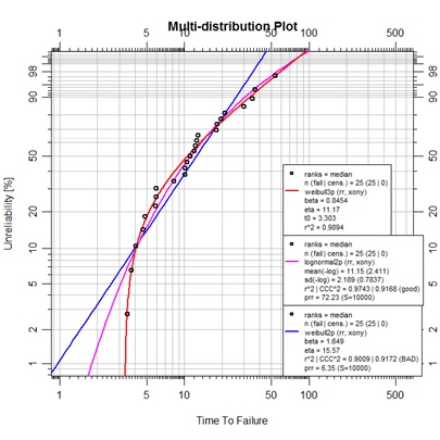
This is a somewhat unexpected display. The example was specifically provided as a lognormal representation, but we observe a much more convincing curve fit with the 3-parameter Weibull. A little examination with SuperSMITH reveals that use of the PVE for fit selection will favor the lognormal (due to a somewhat penalized 3p Weibull MC pivotal determination), but if fitting is performed using MLE, the likelihood ratio test reveals a 90% significance for the 3p Weibull over the lognormal. The abrem package is neutral on this topic as of yet. For now, there is no CCC^2 nor prr value displayed for the 3-parmameter model. In the future provision of a log-likelihood value is expected as a goodness-of-fit measure even for models fit by rank regression.

At times sets of component life data can be too large for simple navigation in a spreadsheet. The next set of data is provided as plain text in a .csv file, which can be read into R for further processing This file can be downloaded using this link.  da.csv
For uniform example it is suggested that this file be placed in a C:\temp\ folder location. The appropriate script for reading this single column of data is provided below. This method would have been the same for a .txt file as well however your browser would have displayed, not downloaded, the file.

daDF<-read.table("C:/temp/da.csv")
da<-as.vector(daDF[,1])

#

Notice the reverse direction of the slashes in the file folder naming here. This is a bit of POSIX legacy. Also, the read.table() function will load the data into a dataframe of only one column in this case. This is then converted to a vector for our purposes. Now, with the data entered, the script for abrem use follows:

#

require(abrem)
dafit<-Abrem(da)
dafit<-abrem.fit(dafit,col="red")
plot(dafit, main="Bathtub Life Data") 

#

Followed by these next lines adding
vertical marker lines. 

#

abline(v=107, col="orange", lty=5, lwd=2)
abline(v=1750, col="orange", lty=5, lwd=2)

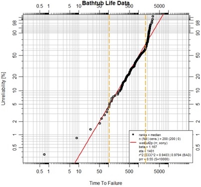
This complete set of life data fits poorly as a Weibull. Not only is the prr less than 10, it is even less than 1.0! We observe, however that the data takes on somewhat expected behavior at the extremes of life. An early period of “infant mortality” appears to give way to a more uniform life profile. Finally, at some later point it appears that wear-out is ultimately over whelming. The orange vertical markers have been placed simply by eye, with some added help of examination of the data in the vicinity of the markers. In accordance with this observation, the data set is split into three parts for examination as 3-parameter Weibulls. Each segment of life data, so divided, is treated as representing a mode of failure; the other segments of data are considered as suspension data for that particular mode.

earlyda<-da[1:10]
midda<-da[11:131]
endda<-da[132:200]
da<-as.vector(daDF[,1])

#

earlyfit<-abrem.fit(Abrem(fail=earlyda,
susp=c(midda,endda),dist="weibull3p"),
col="orange")

#

midfit<-abrem.fit(Abrem(fail=midda,
susp=c(earlyda,endda),dist="weibull3p"),
col="magenta")

#

endfit<-abrem.fit(Abrem(fail=endda,
susp=c(earlyda,midda),dist="weibull3p"),
col="blue")

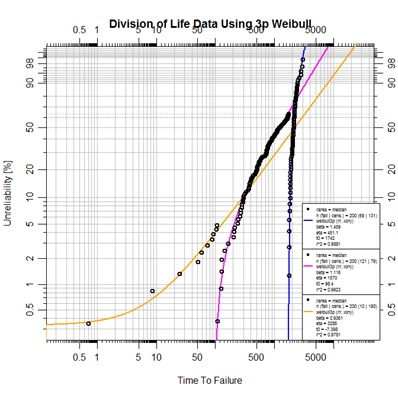
plot.abrem(list(earlyfit,midfit,endfit), legend.text.size=0.5,
main="Division of Life Data Using 3p Weibull") 

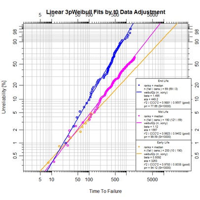
The resulting plot demonstrates much closer fitting to the segmented data. Currently abrem objects will only plot actual data points, not points modified by subtraction of t0. In order to prepare an alternate view depicting the linear fit of these three life-mode segments the next script has been prepared. This script calls on the same underlying function in package pivotals that abrem calls in order to identify the t0 value. Yes, one could have viewed these values from the legend of the last plot and proceeded by utilizing those observed t0 values as constants, but this script has an elegance of working directly off the data itself.

One may note the negative t0 value for the early data upon evaluation for the 3rd parameter. This may suggest some kind of pre-wear or pre-stress placed on the component before it was placed in service. It is not wise to ignore 3-parameter a fit with negative t0. A review of the physics of failure may yield a plausible explanation. In this case the component was the diaphragm on an acid gas compressor. Further review resulted in changes to maintenance methods for installing this component.

## pivotals function MRRw3pxy is to be
## depreciated in favor of MRRw3p
earlyw3pfit<-MRRw3p(earlyda,c(midda,endda))
earlyt0<-earlyw3pfit[3]
earlymodfit<-abrem.fit(Abrem(
fail=(earlyda-earlyt0),
susp=c((midda-earlyt0),(endda-earlyt0)),
col="orange"),label="Early Life") 

#

midw3pfit<-MRRw3p(midda,c(earlyda,endda))
midt0<-midw3pfit[3]
midmodfit<-abrem.fit(Abrem(
fail=(midda-midt0),
susp=(endda-midt0),
col="magenta"),label="Mid Life") 

#

endw3pfit<-MRRw3p(endda,c(earlyda,midda))
endt0<-endw3pfit[3]
endmodfit<-abrem.fit(Abrem((endda-endt0),
col="blue"),label="End Life") 

#

plot.abrem(list(earlymodfit,midmodfit,endmodfit),legend.text.size=0.6,
main="Linear 3p Weibull Fits by t0 Data Adjustment") 

At this time MLE fitting has only rudimentarily been implemented in the abrem package. It is possible to assign method.fit options of either “mle” or “mle-rba” to a 2-parameter Weibull abrem object, only. A simple example is drawn from Appendix C of the text using the very small example data set found there.

require(abrem)
mle_ex<-Abrem(
fail=c(1500,2250,4000,4300,7000),
susp=c(1750,5000))  
mle_ex<-abrem.fit(mle_ex,
method.fit="mle", col="blue")
mle_ex<-abrem.fit(mle_ex,
method.fit="mle-rba", col="purple")
plot(mle_ex, xlim=c(500,10000),
main="MLE and MLE-RBA Fitting")

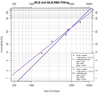
Further development with MLE contours and likelihood ratio bounds is available in the underlying debias package. This is one of the frontiers of the Abernethy Reliability Methods project.

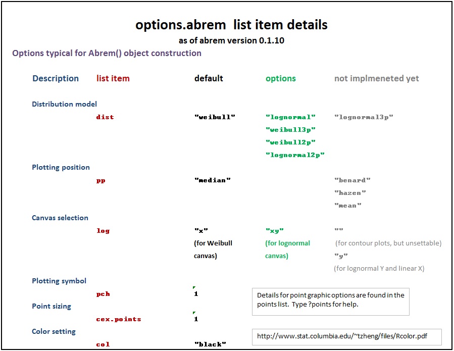
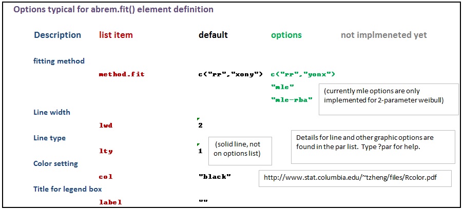
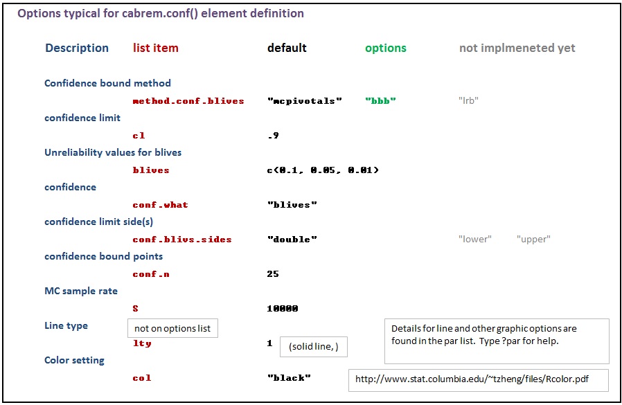
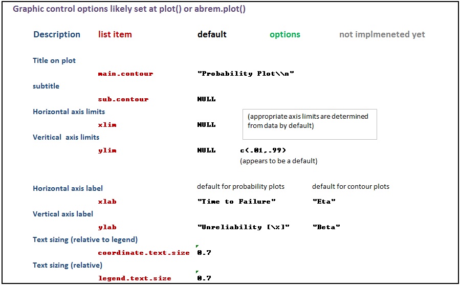
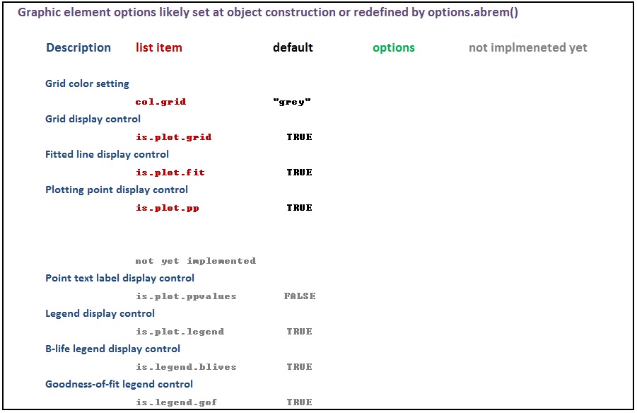
The various options used as named arguments to the Abrem() constructor function, the two element addition methods, abrem.fit() and abrem.conf(), and the plot() or plot.abrem() functions are selected from a list of options available for implementation within abrem. While it is generally possible to add these option arguments in any of the above function calls, there is a certain local applicability of each option to specific steps of object creation and display. Options entered during object definition and display in this way do not persistently alter the default list, but graphic settings will carry though a given object definition until changed again. The following list has been prepared to assist understanding of the options.abrem list. Clicking on the first image will initiate a download of the Excel file used to generate these images.

It is possible to alter the default list for a session or series of related scripts to avoid repetitious argument placement in individual scripts. When this is done it is recommended to store the default list before such alteration and returning the defaults when done.

The following example code sets the default distribution model to lognormal, using the lognormal canvas, and Benard’s approximation for plotting position ranking (to match some commercial software product defaults, perhaps).

default.options<-options.abrem()
options.abrem(dist=”lognormal”, log=”xy”, method.fit=”benard”)

After such a session the following restoration code is recommended.

options.abrem(default.options)

Alteration of the options.abrem list is not recommended within any specific object definition script.