Kettelle's Algorithm

The study of parts supply optimization is best started at the place that first interested Jorge Fukuda; the example problem found in Chapter 7, Section 4 of &  “Statistical Theory of Reliability and Life Testing”, by Richard E. Barlow and Frank Proschan. I was fortunate to find a very inexpensive used copy of this older book (1975) in order to follow along.

This initial problem has the simplest set of conditions for an inventory optimization. The maintenance depot at a single base is required to supply spare parts for immediate installation on some active service assembly (like an aircraft). The maintenance depot receives the failed part and can repair it in a known period of time. Such repaired parts are then available as valid spare parts for another failure instance. The depot or base is considered an echelon, so this is a single echelon problem. Each part is singular, that is there are no sub-assemblies to the part needing repair, so this is a single indenture problem as well.

In order to attempt to have parts available upon failure, there must be some stock inventory for each part; else any part in failure would have to wait for the entire part repair activity to complete. In a pure statistical sense there can never be enough parts in initial stock inventory to always assure a part is on hand when needed. So, a measure of depot performance in its mission can be the probability that a part will be on hand when needed. This is called the Fill Rate in the text. If no spare parts are held, this probability will be zero. As an infinite number of parts are held, this probability will approach 100 percent.

For each part the Fill Rate will be the frequency of having a specific part on hand when a failure occurs divided by the sum of frequencies for all part fail rates. Since the denominator is a constant for any collection of parts, a simplification is made to calculate only the numerator of the Fill Rate function; this is referred to this as the Fill Rate Numerator (FRN). Since part failures are assumed to occur randomly, the Poisson distribution is used. The FRN will be a function of the part fail rate, the time required to repair each part, and the number of replacements intended to be stocked as spares for this part. The individual FRN values are additive-separable, that is we can simply add the incremental FRN value for a specific part addition to the combined FRN contributions of all other parts in an allocation. By magic of Palm’s Theorem this FRN equation is determined for us; we really do not have to derive it for ourselves. Extended reading in Jorge Fukuda’s site on this point can be a plus. 

Parts have a cost, and holding some number of them will consume a budget. So, the Kettelle algorithm is a way to identify the optimal performance measure for the depot given any specific budget for spare parts that can be held.

For simplicity of example, this problem considers only 4 part types. Of course a real maintenance situation would likely consider hundreds or thousands of parts. The solution starts with no stocked parts at all, resulting in a performance measure of zero. As parts are added to the initial stores, performance improves at some cost. As each part is added, an examination is made as to whether the performance measure is the best at that cost or below. The set of varied part quantities that is optimal at a given cost level is considered an Un-dominated Allocation. As un-dominated allocations are identified, all lesser performing combinations of part quantities are Excluded Allocations. An iterative process is performed to go through all likely quantities of each part in combination with quantities of the other parts seeking the combinations of part quantities (the Allocations) that are Un-Dominated. Some part allocations may appear to be un-dominated in the order encountered, but ultimately are found to be dominated by some later trial.

Since Kettelle’s algorithm tests all incremental additions of parts to identify Un-dominated part quantities, it is relatively computationally time consuming, perhaps too much so for practical use in a large scale problem. However, it will identify all un-dominated allocations, and by study of this method we understand the concept of this kind of optimization.

To initiate the solution, the example data has been placed in the xmetric package as a dataframe named Barlow.Proschan. A small function, FRN(), is an implementation of the Fill Rate Numerator calculation that will be called repetitiously from the solution code.

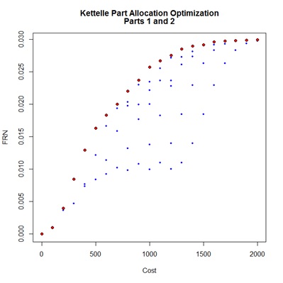
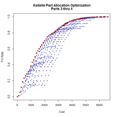
The algorithm is completed in a function named Kettelle() taking a dataframe, having the same form as the example data, as primary argument. A default limit value may be altered to control the extent of the evaluation. The output is a dataframe listing the Un-dominated Allocations containing the quantity of parts by type the total Cost and the resultant Performance measure for each allocation selection. With an argument value of show=TRUE a graphic display will appear showing the Un-dominated Allocations as red points and the Excluded Allocations as blue. A name label can be provided as an identifier in the chart title. Further, the performance measure may be selected to represent “FRN” (as default), “Fill Rate”, or “EBO” as to be discussed later.

The heart of this General Kettelle Algorithm (GKA, in the text) is a triple-nested loop going through all parts, all Un-dominated Allocations previously identified, and all quantities of each successive part that generate incremental performance improvement greater than the set limit. As each new quantity of each part is encountered a series of logic blocks determine whether this addition represents a new Un-dominated Allocation, and if so whether it identifies existing entries in the pending UdomAll dataframe as Excluded.

The result of interest to a depot manager is the sequence of Un-dominated Allocations. From this series, expressed as red dots here, the required budget for a target Fill Rate can be established, or alternatively, the likely Fill Rate to be expected given a fixed budget. The specific stock quantities of each part required to achieve the optimal budgetary values is identified.

Use of the Kettelle() function is very simple. First, some data must be identified. The small example dataset of 4 parts used by Barlow and Proschan has been incorporated into the xmetric package as a dataframe named Barlow.Proschan.

The package library must be loaded once for an R session. Then the desired data built into the package must be loaded for use.

#

require(xmetric)
data(Barlow.Proschan)

#

With the data loaded we can call the Kettelle function with some qualifying arguments. Here the data has been subveiwed to handle only parts 1 and 2.

#

parts1and2<-Kettelle(Barlow.Proschan[1:2,],data.name = "Parts 1 and 2",show=TRUE)
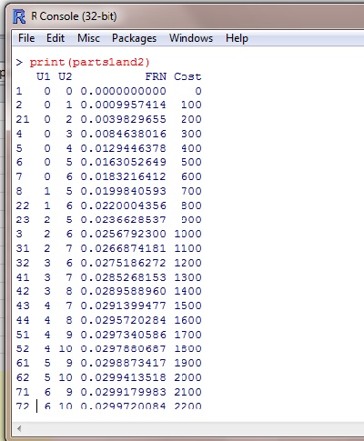
print(parts1and2)

#

By assigning a label for the ouput object of this function, the UdomAll dataframe will be stored in session memory. This object can then be printed in the R console, from where it might be copied and pasted into a spreadsheet for instance. Once the text of the output is placed in Excel a Data…Text_to_Columns command sequence will bring up a dialog to place the table in a more useable form.

#

Similar steps could be taken to examine parts 3 and 4, or parts 1 through 4 as Fukuda has demonstrated. Use of the "Fill Rate" performance measure simply alters the performance scale and values, the graphic is unchanged.

The Fill Rate performance measure used so far in the Kettelle part allocation optimization does not reflect the full impact of not having a part upon demand, because it does not reflect the resulting waiting time that may be required to eventually deliver the part. A better measure is defined as the Estimated Back Orders, or EBO. This measure correlates with the average waiting time for unfilled demands. For the case where there are no spares held this will be the product of demand rate and repair turnaround time on an individual part basis. This product is referred to as the pipeline, and is designated PL, below. As spares are held in increasing quantities, the EBO measure will decrease, approaching zero as spare holdings approach infinity.

After study through various texts, it has been found very difficult to generate this function in computer programmable terms given theoretical presentations. However, Jorge Fukuda has very elegantly presented this function in terms of an Excel formula:

               
            EBO = PL * POISSON (s, PL, FALSE ) + (PL − s) * [1− POISSON (s, PL,TRUE)]

, where 
PL is the pipeline value determined by demand rate * turnaround time, and
s   is the quantity of initial spares in stock. 

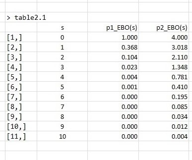
As expected, the EBO is a function based on the Poisson distribution where the PL value is diminished as spare holdings increase. This EBO function has also been added to the xmetric package. The source code for this function can be viewed by simply typing EBO at the R command prompt, assuming the xmetric library has been loaded. A test of this function now implemented in R permits replication of a reference Table 2-1 in Sherbrooke’s text, giving further confidence in its use.

require(xmetric)
p1<-c(Lam=10,TAT=0.1)
p2<-c(Lam=50,TAT=0.08)
table2.1<-matrix(nrow=11,ncol=3,rep(0,11*3))
for(s in 0:10) {
table2.1[s+1,1]<-s
table2.1[s+1,2]<-round(EBO(s,p1[1],p1[2]),3)
table2.1[s+1,3]<-round(EBO(s,p2[1],p2[2]),3)
}
colnames(table2.1)<-c("s","p1_EBO(s)","p2_EBO(s)")
print(table2.1)

#

As with the FRN performance measure, EBO contributions are additive. Incremental differences due to additions to stock are additive, albeit negative values.

The optimization of EBO performance is a minimization rather than the maximization required with FRN, so the Kettelle() function needs to handle this addition. This is done by adding the modified code for the minimization as a separate block after a conditional test for the direction of optimization as of version 0.0.3 of the xmetric package.

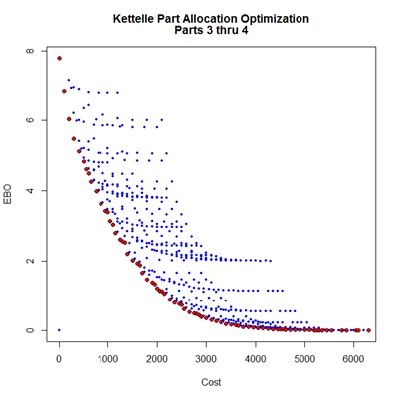
The following scripts present analysis of all 4 parts in the example set according to the “EBO” and “Fill Rate” performance measures. The results appear to be a reflection about an ultimate performance horizontal; however examination of the un-dominated allocation tables would reveal some differences in part selections. Alteration of the limit value between the two measures is required to maintain similar extent of study.

#

#

#

require(xmetric)
data(Barlow.Proschan)
Kettelle(Barlow.Proschan,
data.name="Parts 3 thru 4",
performance="EBO", limit=10^-2.5,
show=TRUE)

#

#

#

#

#

#

#

#

#

#

#

#

#

#

#

require(xmetric)
data(Barlow.Proschan)
Kettelle(Barlow.Proschan,
data.name="Parts 3 thru 4",
performance="Fill Rate", 
show=TRUE)

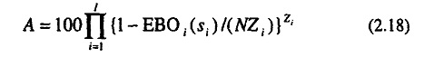
It is possible to derive a system measure of availability from the EBO measures for each part, but this depends on the number of active parts in the system; a bit of data that has not been provided with our reference examples. Sherbrooke provides the following equation for an availability determination for a system of N aircraft each having a quantity of Z active parts.

This is but a launch point for further reusable part optimization studies. The code is open source and you are encouraged to review it. Someone else may come up with a more elegant set of logic steps for identification of the un-dominated allocations; if so, please let us know. If this were to become part of a real production application, conversion of the code to C++ using Rcpp would be expected to improve execution speed dramatically. As is, the code is quite responsive for this simple example.